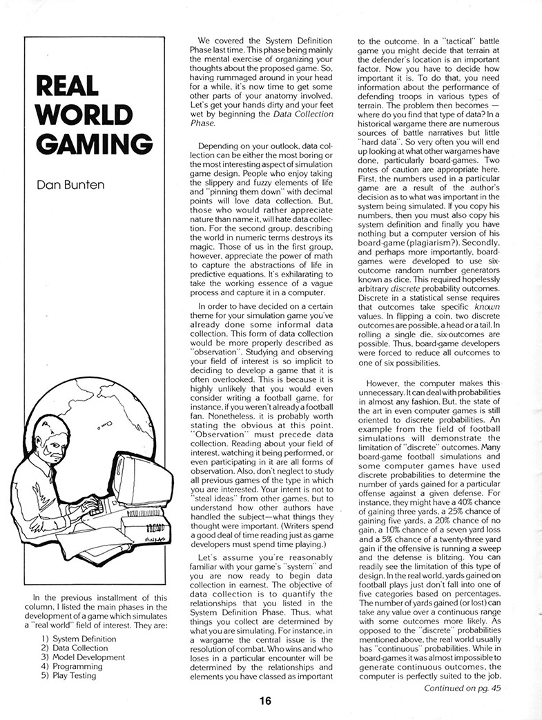
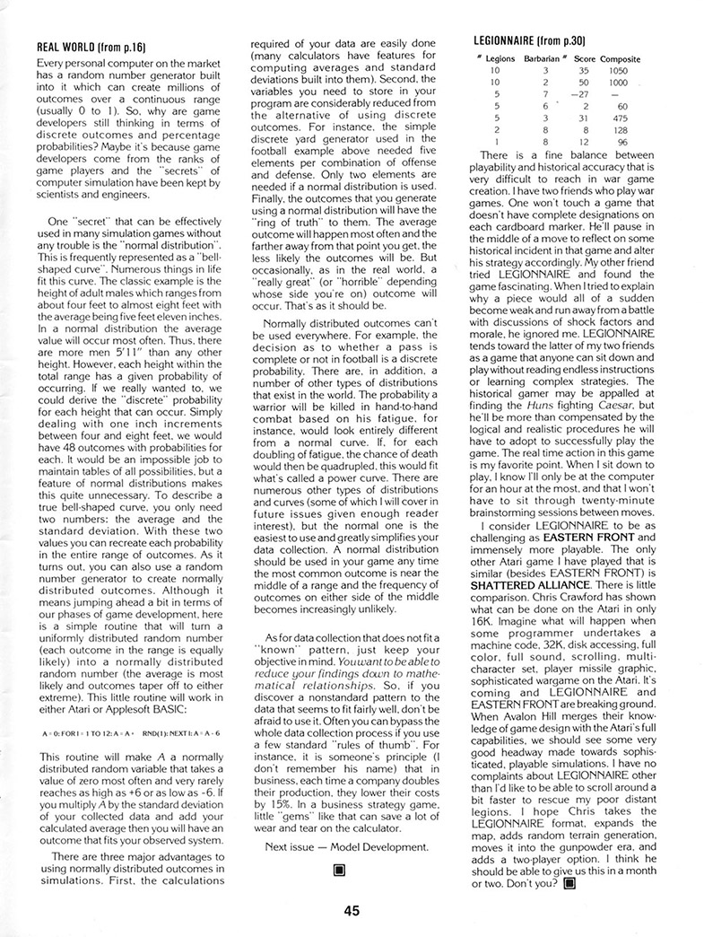
Real World Gaming

In the previous installment of this column, I listed the main phases in the development of a game which simulates a “real world” field of interest. They are:

1) System Definition
2) Data Collection
3) Model Development
4) Programming
5) Play Testing

We covered the System Definition Phase last time. This phase being mainly the mental exercise of organizing your thoughts about the proposed game. So, having rummaged around in your head for a while, it’s now time to get some other parts of your anatomy involved. Let’s get your hands dirty and your feet wet by beginning the Data Collection Phase.

Depending on your outlook. data collection can be either the most boring or the most interesting aspect of simulation game design. People who enjoy taking the slippery and fuzzy elements of life and “pinning them down” with decimal points will love data collection. But, those who would rather appreciate nature than name it. will hate data collection. For the second group. describing the world in numeric terms destroys its magic. Those of us in the first group, however. appreciate the power of math to capture the abstractions of life in predictive equations. It’s exhilarating to take the working essence of a vague process and capture it in a computer.

In order to have decided on a certain theme for your simulation game you’ve already done some informal data collection. This form of data collection would be more properly described as “observation”. Studying and observing your field of interest is so implicit to deciding to develop a game that it is often overlooked. This is because it is highly unlikely that you would even consider writing a football game, for instance, if you weren’t already a football fan. Nonetheless. it is probably worth stating the obvious at this point. “Observation” must precede data collection. Reading about your field of interest. watching it being performed, or even participating in it are all forms of observation. Also. don’t neglect to study all previous games of the type in which you are interested. Your intent is not to “steal ideas” from other games. but to understand how other authors have handled the subject — what things they thought were important. (Writers spend a good deal of time reading just as game developers must spend time playing.)

Let’s assume you’re reasonably familiar with your game’s “system” and you are now ready to begin data collection in earnest. The objective of data collection is to quantify the relationships that you listed in the System Definition Phase. Thus. what things you collect are determined by what you are simulating. For instance, in a wargame the central issue is the resolution of combat. Who wins and who loses in a particular encounter will be determined by the relationships and elements you have classed as important to the outcome. In a “tactical” battle game you might decide that terrain at the defender’s location is an important factor. Now you have to decide how important it is. To do that, you need information about the performance of defending troops in various types of terrain. The problem then becomes — where do you find that type of data? In a historical wargame there are numerous sources of battle narratives but little “hard data”. So very often you will end up looking at what other wargames have done, particularly board-games. Two notes of caution are appropriate here. First, the numbers used in a particular game are a result of the author’s decision as to what was important in the system being simulated. If you copy his numbers. then you must also copy his system definition and finally you have nothing but a computer version of his board-game (plagiarism?). Secondly, and perhaps more importantly, boardgames were developed to use six-outcome random number generators known as dice. This required hopelessly arbitrary discrete probability outcomes. Discrete in a statistical sense requires that outcomes take specific known values. In flipping a coin, two discrete outcomes are possible. a head or a tail. In rolling a single die. six-outcomes are possible. Thus. board-game developers were forced to reduce all outcomes to one of six possibilities.

However, the computer makes this unnecessary. It can deal with probabilities in almost any fashion. But. the state of the art in even computer games is still oriented to discrete probabilities. An example from the field of football simulations will demonstrate the limitation of “discrete” outcomes. Many board-game football simulations and some computer games have used discrete probabilities to determine the number of yards gained for a particular offense against a given defense. For instance, they might have a 40% chance of gaining three yards. a 25% chance of gaining five yards. a 20% chance of no gain, a 10% chance of a seven yard loss and a 5% chance of a twenty-three yard gain if the offensive is running a sweep and the defense is blitzing. You can readily see the limitation of this type of design. In the real world, yards gained on football plays just don’t fall into one of five categories based on percentages. The number of yards gained (or lost) can take any value over a continuous range with some outcomes more likely. As opposed to the “discrete” probabilities mentioned above. the real world usually has “continuous” probabilities. While in board-games it was almost impossible to generate continuous outcomes, the computer is perfectly suited to the job. Every personal computer on the market has a random number generator built into it which can create millions of outcomes over a continuous range (usually 0 to 1). So, why are game developers still thinking in terms of discrete outcomes and percentage probabilities? Maybe it’s because game developers come from the ranks of game players and the “secrets” of computer simulation have been kept by scientists and engineers.

One “secret” that can be effectively used in many simulation games without any trouble is the “normal distribution”. This is frequently represented as a “bell-shaped curve” Numerous things in life fit this curve. The classic example is the height of adult males which ranges from about four feet to almost eight feet with the average being five feet eleven inches. In a normal distribution the average value will occur most often. Thus, there are more men 5’11” than any other height. However, each height within the total range has a given probability of occurring. If we really wanted to, we could derive the “discrete” probability for each height that can occur. Simply dealing with one inch increments between four and eight feet, we would have 48 outcomes with probabilities for each. It would be an impossible job to maintain tables of all possibilities, but a feature of normal distributions makes this quite unnecessary. To describe a true bell-shaped curve, you only need two numbers: the average and the standard deviation. With these two values you can recreate each probability in the entire range of outcomes. As it turns out, you can also use a random number generator to create normally distributed outcomes. Although it means jumping ahead a bit in terms of our phases of game development, here is a simple routine that will turn a uniformly distributed random number (each outcome in the range is equally likely) into a normally distributed random number (the average is most likely and outcomes taper off to either extreme). This little routine will work in either Atari or Applesoft BASIC:

A = 0: FOR I = 1 TO 12: A = A + RND(1): NEXT I: A = A - 6

This routine will make A a normally distributed random variable that takes a value of zero most often and very rarely reaches as high as +6 or as low as -6. If you multiply A by the standard deviation of your collected data and add your calculated average then you will have an outcome that fits your observed system.

There are three major advantages to using normally distributed outcomes in simulations. First, the calculations required of your data are easily done (many calculators have features for computing averages and standard deviations built into them). Second, the variables you need to store in your program are considerably reduced from the alternative of using discrete outcomes. For instance, the simple discrete yard generator used in the football example above needed five elements per combination of offense and defense. Only two elements are needed if a normal distribution is used. Finally, the outcomes that you generate using a normal distribution will have the “ring of truth” to them. The average outcome will happen most often and the farther away from that point you get. the less likely the outcomes will be. But occasionally, as in the real world. a “really great” (or “horrible” depending whose side you’re on) outcome will occur. That’s as it should be.

Normally distributed outcomes can’t be used everywhere. For example, the decision as to whether a pass is complete or not in football is a discrete probability. There are, in addition. a number of other types of distributions that exist in the world. The probability a warrior will be killed in hand-to-hand combat based on his fatigue, for instance. would look entirely different from a normal curve. If. for each doubling of fatigue, the chance of death would then be quadrupled, this would fit what’s called a power curve. There are numerous other types of distributions and curves (some of which I will cover in future issues given enough reader interest). but the normal one is the easiest to use and greatly simplifies your data collection. A normal distribution should be used in your game any time the most common outcome is near the middle of a range and the frequency of outcomes on either side of the middle becomes increasingly unlikely.

As for data collection that does not fit a “known” pattern, just keep your objective in mind. You want to be able to reduce your findings down to mathematical relationships. So, if you discover a nonstandard pattern to the data that seems to fit fairly well. don’t be afraid to use it. Often you can bypass the whole data collection process if you use a few standard “rules of thumb”. For instance, it is someone’s principle (I don’t remember his name) that in business, each time a company doubles their production, they lower their costs by 15%. In a business strategy game, little “gems” like that can save a lot of wear and tear on the calculator.

Next issue — Model Development.