The Silicon Cerebrum

APOLOGIES

Before getting into this column’s topic, I need to issue a number of apologies. First, I want to apologize for not having a column last issue. Second. to apologize for not covering in this column what I said would be last time. And most of all, I want to apologize to all of you who took me up on my rash offer and wrote for program listings of the algorithm. I really do plan to reply to all of you and to write the promised column. During the last three months, I have changed jobs. changed houses, and have been working under a number of deadlines which have left me little time for doing this column (or many other things). Most of the pressure should be off within a few weeks, so I should be able to get back to these unfinished matters.

A DECISION MAKING METHOD

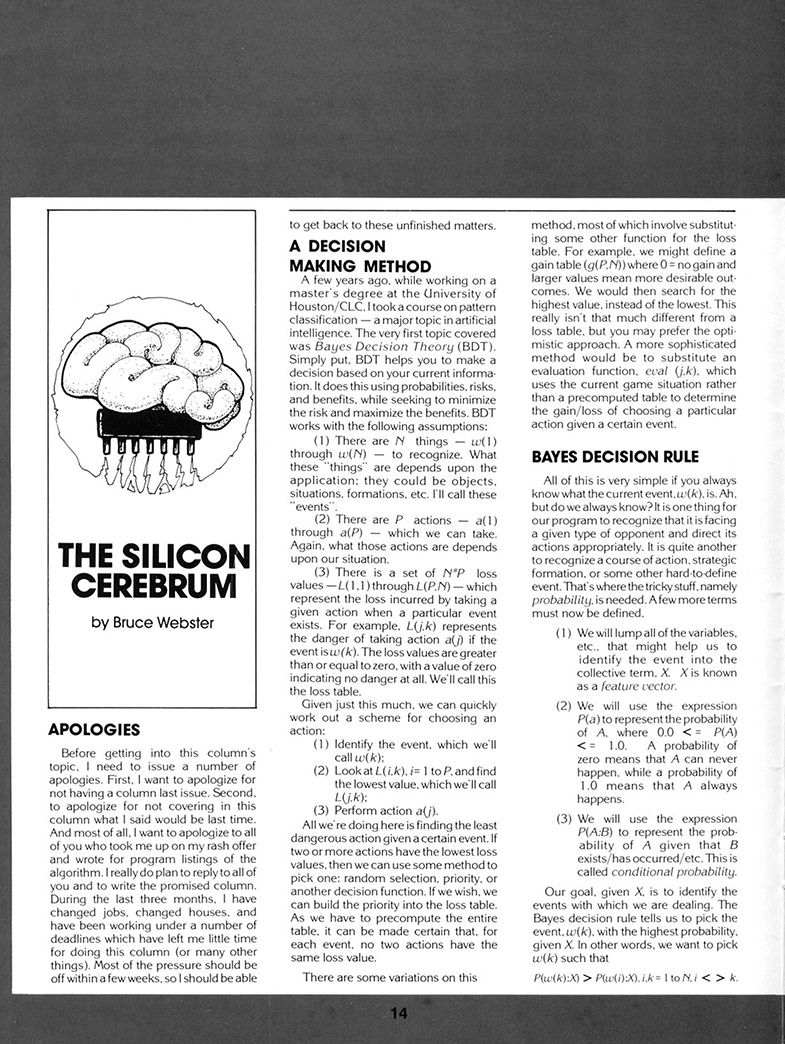
A few years ago. while working on a master’s degree at the University of Houston/CLC, I took a course on pattern classification — a major topic in artificial intelligence. The very first topic covered was Bayes Decision Theory (BDT). Simply put, BDT helps you to make a decision based on your current information. It does this using probabilities, risks, and benefits, while seeking to minimize the risk and maximize the benefits. BDT works with the following assumptions:

(1) There are N things — w(1) through w(N) — to recognize. What these “things” are depends upon the application: they could be objects, situations, formations, etc. I’ll call these “events”.

(2) There are P actions — a(1) through a(P) — which we can take. Again, what those actions are depends upon our situation.

(3) There is a set of N*P loss values — L(1,1) through L(P,N) — which represent the loss incurred by taking a given action when a particular event exists. For example, L(j,k) represents the danger of taking action a(j) if the event is w(k). The loss values are greater than or equal to zero, with a value of zero indicating no danger at all. We’ll call this the loss table.

Given just this much, we can quickly work out a scheme for choosing an action:

(1) Identify the event, which we’ll call w(k);

(2) Look at L(i,k), i = 1 to P, and find the lowest value. which we’ll call L(j,k);

(3) Perform action a(j).

All we’re doing here is finding the least dangerous action given a certain event. If two or more actions have the lowest loss values, then we can use some method to pick one: random selection, priority, or another decision function. If we wish, we can build the priority into the loss table. As we have to precompute the entire table, it can be made certain that, for each event. no two actions have the same loss value.

There are some variations on this method. most of which involve substituting some other function for the loss table. For example. we might define a gain table (g(P,N)) where 0 = no gain and larger values mean more desirable outcomes. We would then search for the highest value, instead of the lowest. This really isn’t that much different from a loss table, but you may prefer the optimistic approach. A more sophisticated method would be to substitute an evaluation function, eval (j,k). which uses the current game situation rather than a precomputed table to determine the gain/loss of choosing a particular action given a certain event.

BAYES DECISION RULE

All of this is very simple if you always know what the current event, w(k), is. Ah, but do we always know? It is one thing for our program to recognize that it is facing a given type of opponent and direct its actions appropriately. It is quite another to recognize a course of action, strategic formation, or some other hard-to-define event. That’s where the tricky stuff, namely probability, is needed. A few more terms must now be defined.

(1) We will lump all of the variables, etc., that might help us to identify the event into the collective term, X. X is known as a feature vector.

(2) We will use the expression P(a) to represent the probability of A, where 0.0 <= P(A) <= 1.0. A probability of zero means that A can never happen, while a probability of 1.0 means that A always happens.

(3) We will use the expression P(A:B) to represent the probability of A given that B exists/has occurred/etc. This is called conditional probability.

Our goal, given X, is to identify the events with which we are dealing. The Bayes decision rule tells us to pick the event, w(k), with the highest probability. given X. In other words, we want to pick w(k) such that

P(w(k):X) > P(w(i):X),i,k = 1 to N,i < > k.

(As before, we may need a tie-breaking method in case there are some identical maximum probabilities.)

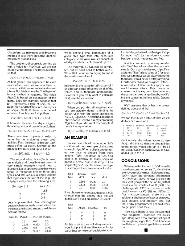
The problem, of course, is coming up with a value for P(w(i):X). We are not entirely without help. The Bayes rule tells us that

P(w(i):X) = P(X:w(i)) * P(w(i)) / P(X).

At first glance, this appears to be even more of a mess, for we now have to come up with three sets of values instead of one. But this is where the “intelligence” in our method is required. The value P(w(i)) is based on observation of the game. Let’s, for example, suppose that w(i) represents a type of ship that we might face, and that there are three types of ships (N=3). If there is an equal number of each type of ship. then

P(w(1)) = P(w(2)) = P(w(3)) = 0.333.

If, however, there are five ships of type 1, three of type 2, and one of type 3, then

P(w(1)) = 0.5, P(w(2)) = 0.3, and P(w(3)) = 0.2

There are two important rules to remember in assigning these probabilities. First, the set w(1) through w(N) must define all cases. Second, all the probabilities must add up to 1.0, or

sum[P(w(i)), i = 1 to N] = 1.0.

The second value, P(X:w(i)). is based on analysis and (possibly) test cases. A very simple example should help to illustrate. Let’s suppose again that we are trying to recognize one of three ship types, and that Xis just a single variable that represents the size of the ship. The ship types may have the following sizes:

Ship type (w)	Sizes (X)
1	1,2,3
2	2,3
3	3,4

Let’s suppose that observation/game design/whatever leads us to believe that the ships are divided among the different sizes as follows:

Sizes (X)	P(X:w(1))	P(X:w(2))	P(X:w(3))
1	0.5	0.0	0.0
2	0.333	0.333	0.0
3	0.167	0.5	0.167
4	0.0	0.167	0.833

We’re defining what percentage of a given ship type falls into each size category. so the values must account for all ships and each column add up to 1.

The third value, P(X), can be computed, but we don’t need to bother with it. Why? Well, what we are trying to find is the maximum value of

P(w(i):X) for i = 1 to N, P(X).

however, is the same for all values of i, so it has an equal influence on all of the values and is therefore unimportant. However, if you really want to calculate P(X), use the expression

P(X) = sum[P(X:w(i))*P(w(i)), i = 1 to N].

When you put this all together. what you are actually doing is finding the action, a(j). with the lowest associated risk, R(j), given X. The method described above doesn’t involve directly computing R(j), but if you did want to compute it, here’s the expression:

R(j) = sum[L(j,i)*P(w(i):X), i = 1 to N].

AN EXAMPLE

To see how this all fits together, let’s continue with our example of the three types of ships. When a ship is encountered, we have to choose from three actions: fight, negotiate, or flee. Our goal is to destroy as many ships as possible before ours is destroyed. Our ship is of type 2; type 1 is weaker and type 3 is stronger. Here are our attack odds:

Ship type	Enemy dest.	Both dest.	Us dest.
1	0.666	0.333	0.0
2	0.333	0.333	0.333
3	0.0	0.333	0.666

If we choose to negotiate, there is a 50% chance that the enemy ship will not attack. Let’s build an ad hoc loss table:

Ship type	Attack	Negotiate	Flee
1	4	6	5
2	5	5	5
3	6	6	5

As this is set up, we will always attack a type 1 ship and always flee a type 3 ship. We will use some sort of decision function for deciding what to do with a type 2 ship; for now, we’ll just randomly choose between attack, negotiate, and flee.

A side comment: you may wonder why “flee” has a loss value. the reason is simple. Our goal is to destroy ships. If we assigned “flee” a loss value of 0 for each ship type, then we would always flee and, therefore, would never destroy anything. If, on the other hand, we assigned “attack” a loss value of 0 for each ship type. we would always attack. This means, of course, that the way our ship acts during the game can be changed just by modifying the values in loss table. Getting any ideas?

We’ll assume that X has the values defined above and that

P(w(1)) = 0.5, P(w(2)) = 0.3, and P(w(3)) = 0.2.

We can then build a table of what we will do for each value of X.

X	P(w(1):X)	P(w(2):X)	P(w(3):X)	type	action
1	1.0	0.0	0.0	1	attack
2	0.625	0.375	0.0	1	attack
3	0.313	0.562	0.125	2	select
4	0.0	0.232	0.768	3	flee

(Incidentally, the values above do use P(X). I did this so that the probabilities going across would add up to 1. Had I not used P(X), then each row would have added up to P(X).)

CONCLUSIONS

When you think about it. BDT is really based on common sense. To identify the event, you pick the most likely candidate, (w(k)) given the pertinent information (X). Once you know (or have guessed at) the event, you pick the action (a(j)) that results in the smallest loss (L(j,k)). The challenge with BDT is to come up with useful values for P(w(i)) and P(X:w(i)). For microcomputers. there are the additional challenges of execution speed, data storage, and program size. But that’s why programmers get paid (they do get paid, don’t they?).

Next issue, I hope to have the weighted map diagrams I promised two issues ago, along with a few example listings of the weighting algorithm. And, I hope to finally have my backlog of letters cleared out.